
- Global climate is always changing!
- Temperature is a dynamic cyclical process
- The rocks are the record
- The Earth is a dynamic system
- “The biochemical-geophysical Greenhouse”
- Climate drivers
- Second-order climate controls
- Fourth-order climate controls
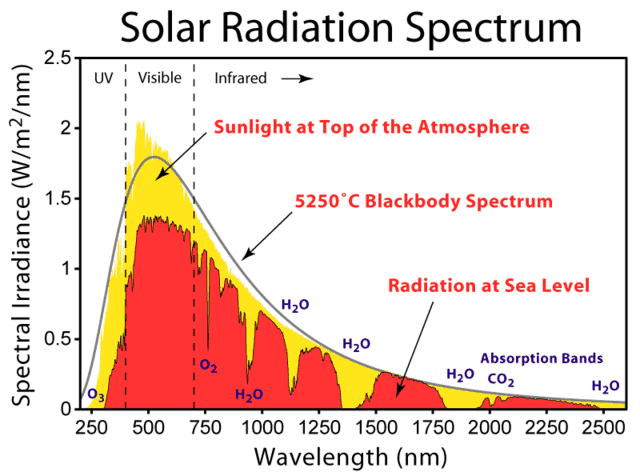
- The Sun is the primary energy source for climate on earth
- Albedo
- Irradiance—incident solar energy—varies
- Solar Activity Cycles from 1749
- Solar activity affects climate
- The solar magnetic activity cycle
- Sunspots
- Sunspots and Wolf numbers
- Solar activity proxies
- Dendroclimatology
- Milankovitch Cycles and Glaciation
- The 100,000 year Milankovitch cycle:eccentricity
- The 41,000 year Milankovitch cycle: axial tilt
- The 23,000 year Milankovitch cycle: precession
- The Energy Budget of the Earth
- The Winds
- The Coriolis force
- The Coriolis effect and ocean currents
- The Sargasso Sea
- Geostrophic balance
- The thermohaline circulation
- Temperature-density effects
- The carbon cycle
- Estimating ancient temperatures
- Reconstructing paleoclimate
- O2 Isotopes as paleoclimate proxies
- Oxygen isotopes, temperature, and weather
- Temperature and isotope ratios
- Paleoclimate from benthic organisms
- Paleoclimate from insects
- Paleoclimate from stomatal index records
- Sea level changes
- Ocean basin changes
- Eustatic sea level changes
- The origins of the CO2 controversy
- The uncontrolled experiment on Western Civilization
Climate Change: The “big” picture
Rational Science without the political rhetoric
Global climate is always changing!
Global climate has been changing since the most primitive atmosphere developed on earth more than 3 billion years ago. It will continue to change so long as the Earth has an atmosphere and the sun continues to shine. Climate change on Earth has been continuous and has occurred on all timescales. Climate change must be considered in the context of geologic time and the history of planet Earth.
Climate change cannot be measured over a human life span. Determining the direction of global temperature change is a function of the time span used to make the determination.
Geological interpretations are four-dimensional
Geology considers time as well as space.
On the 10,000-year interglacial scale, the earth is cooling from the high temperatures of the early interglacial. However, on a 16,000-year record, starting in the late Pleistocene glacial episode, the overall effect is global warming. Similarly, the last 2000 years show that the earth is cooling, over the last 600 years it is slightly warming, and over the last decade it is warming. Picking the time constraint for a model determines the model’s outcome, without regard to the complexity of the model.
Temperature is a dynamic cyclical process!
Global temperatures vary in predictable cycles.

Global temperatures and volcanic activity (2500 bce to 2008 AD)
In relatively recent times, the Medieval Climate Optimum, or Medieval Warm Event (MWE) (a.d.~1200–1350), was the time of castle building, growing vineyards in northern Europe, and the settlement of agricultural colonies by Vikings in Greenland. This warm period in human history was followed by the Little Ice Age (LIA), from the end of the MWE to about 1850, when temperatures plunged sufficiently to isolate the Greenland colonies by sea ice and cause their demise. Society prospered during the MWE, but suffered greatly from starvation, plague, and pestilence during the ensuing cold years.
The human species and all the other animals and plants on Earth can only adapt to inevitable climate change and mitigate its effects during each generation.
Political processes cannot change Earth’s dynamic biogeochemical processes.
All the scientists, engineers, academics, and politicians alive can not stop climate from changing. Adaptation to the changes that continually occur on Earth requires flexibility, planning, and acceptance of the earth-system constraints.
This paper summarizes without rancor and empty, meaningless rhetoric, the critical facts every concerned human being needs to understand and rationally discuss how to mitigate the inevitable effects of climate change .
The rocks are the record
The problem with discussing climate arises from the need to consider time scales and talk about climate during particular time periods. Geology provides the historical context for any rational discussion of climate change on Earth.
The sedimentary rock record reflects numerous sea-level changes, changes in atmospheric composition, and temperature changes, all of which attest to variations in climate. Past climates have varied from those that create continental glaciers to those that yield global greenhouse conditions. The Earth’s climate gets warmer or cooler but typically does not remain the same for extended periods of geologic time. Human history shows us that in general, warmer conditions have been more beneficial to human society than colder conditions.
Today we are living through a not-yet-completed interglacial stage. We have been in this interglacial period for about 10,000 years.
Interglacial periods appear to last for about 11,000 years, but with large individual variability. It is very likely that warmer conditions lie ahead for humanity, with or without any direct human contribution.
Consider the really long term perspective. Climate over the last 500 million years.

Climate, the really long term perspective: 500 million years
Moving to greater detail, consider the last 500 thousand years
 ice core: 500,000 years - Victor John Yannacone, jr")
Vostok (antarctica) ice core: 500,000 years
And refining the time scale further consider those Vostok ice cores over the last 50 thousand years
 ice cores past 50000 years - Victor John Yannacone, jr")
Vostok (Antarctica) ice cores past 50000 years
From the perspective of 500 million years we can prooperly consider the climate of the last 10,000 years.
Human society evolved over the last 10,000 years. For 6000 years it was much warmer than today. Our ancestors enjoyed a much warmer world.

Greenland GISP2 ice core, the last 10,000 years
The period of human history over the last 4500 years.
The Earth has been cooling for 4000 years.

GISP2_temperatures over the last 4,000 years
The Earth is a dynamic system
The earth is a complex dynamic system integrating a number of coupled large complex dynamic systems: the atmosphere, the hydrosphere, the lithosphere and the biosphere. The Earth and all its systems are billions of years old and have never been in equilibrium. The continuing interactions among all these systems of the Earth are responsible for climate on the surface of the earth.
Geology is a scientific discipline that routinely works backward through significant periods of time to understand the natural processes of the Earth as a dynamic system.
Climate can vary rapidly and over a range that can have a profound influence on human society. There are predictable geologic effects from climate change such as sea-level variations, changes in the rates of glacial movement, ecosystem migration, methane hydrate formation, and changes in agricultural productivity. Geologic processes are not in equilibrium and this makes assessing any cumulative human impact on climate difficult. It is difficult to determine the range of natural variation in global climate over the last 10,000 years, and even more difficult to determine the impact of human activities on such variation.
Geology brings both data from the past history of climate and scientific methods for interpreting such data to the discussion about the effect which greenhouse gases from human activities may have on global temperature behavior.
The biochemical-geophysical “Greenhouse”
Human life on Earth exists in a biochemical-geophysical “greenhouse” which has been evolving over more than 4 billion years.
The greenhouse envelope of the atmosphere which evolved over billions of years is the primary temperature control that permits life, as we know it, to exist. Without that envelope, it is likely that the earth’s temperature would be 15°–30°C below its present level.

 - Victor John Yannacone, jr")
Greenhouse gas sources (Gerhard)

The annual carbon budget from all human activities is approximately 2.7–3.4%.

Mars: Not enough greenhouse effect
Not enough greenhouse effect: The planet Mars has a very thin atmosphere, nearly all carbon dioxide. Because of the low atmospheric pressure, and with little to no methane or water vapor to reinforce the weak greenhouse effect, Mars has a largely frozen surface that shows no evidence of life.

Venus: Too much greenhouse effect
Too much greenhouse effect: The atmosphere of Venus, like Mars, is nearly all carbon dioxide. But Venus has about 154,000 times as much carbon dioxide in its atmosphere as Earth and about 19,000 times as much as Mars does, producing a runaway greenhouse effect and a surface temperature hot enough to melt lead.
About 80% to 95% of the total greenhouse gas budget is water vapor (including clouds) and the remainder consists of CO2, methane, and other gases.

Greenhouse gas molecules (NASA)
- Water vapor. The most abundant greenhouse gas, but importantly, it acts as a feedback to the climate. Water vapor increases as the Earth’s atmosphere warms, but so does the possibility of clouds and precipitation, making these some of the most important feedback mechanisms to the greenhouse effect.
- Carbon dioxide (CO2). A minor but very important component of the atmosphere, carbon dioxide is released through natural processes such as respiration and volcano eruptions and through human activities such as deforestation, land use changes, and burning fossil fuels.
- Methane. A hydrocarbon gas produced both through natural sources and human activities, including the decomposition of wastes in landfills, agriculture, and especially rice cultivation, as well as ruminant digestion and manure management associated with domestic livestock. On a molecule-for-molecule basis, methane is a far more active greenhouse gas than carbon dioxide, but also one which is much less abundant in the atmosphere.
-
 Flaring natural gas
(Source: https://www.washingtonpost.com/wp-apps/imrs.php?src=https://arc-anglerfish-washpost-prod-washpost.s3.amazonaws.com/public/EHNGETQOLAI6XNAERUPGOXWHAE.jpg&w=916)
- Nitrous oxide. A powerful greenhouse gas produced by soil cultivation practices, especially the use of commercial and organic fertilizers, fossil fuel combustion, nitric acid production, and biomass burning.
- Chlorofluorocarbons (CFCs). Synthetic compounds entirely of industrial origin used in a number of applications, but now largely regulated in production and release to the atmosphere by international agreement for their ability to contribute to destruction of the ozone layer. They are also greenhouse gases.
Climate drivers: First-, second-, third-, and fourth-order climate controls
Climate drivers vary in intensity and over time.
Human influences are of comparatively low intensity and take place over short time spans. The non-equilibrium systems that control natural phenomena on earth dwarf the ability of human beings to affect climatic conditions on a global scale other than by means of global nuclear or biological war.
The scale of temperature changes through time compared with climate change drivers can be visualized with an ordering of climate drivers and timescales which suggests there is a direct relationship between the range of absolute temperature change and the amount of time over which the climate drivers operate.
In the following graphic, the diamond shapes are interpreted from literature-documented ranges of values and dots indicate possible ranges of values. The error bars for the interpretations are broad, but the phenomena appear to fall into significant categories of effects and time.
The blue diamonds represent the estimated range of values for the named processes which affect surface temperature on the Earth over time.

Climate Effects Duration
The Second Order diamond represents the effects of continental movements and resultant changes in ocean currents occurring over millions to hundreds of million years on temperature. The range is 10°–25° Celsius.
Similarly the third and fourth order diamonds represent smaller effects ocer shorter time scales.
Human effects on climate fall into the very short time and small-scale effects and are the least effective, perhaps one or two degrees over a hundred years.
Climate drivers can be categorized by the range of temperature change forced by the driver and the length of time over which the driver operates. The vertical axis (time) is logarithmic (units are powers of 10), and the horizontal axis (temperature effect/change) is arithmetic. This permits comparison of climate drivers with their potential effects and separation of drivers of different magnitude.
Second-order climate controls
Second-order climate control results from the distribution of continents and oceans upon the planet which controls the major ocean currents which distribute heat. This fundamental concept explains the 15°–20°C temperature variations over hundreds of million of years.
The climate of the Earth has been continuously cycling between glacial “icehouse” and warm “greenhouse” states. The late Precambrian “icehouse” 4600–541 million years ago evolved into the Devonian “greenhouse” which lasted from 419.2–358.9 million years ago followed by the Carboniferous “icehouse” from 358.9–298.9 million years ago then the Cretaceous “greenhouse” from 145–66 million years ago which evolved to the present “icehouse” state. Glacial activity has been identified in the “record of the rocks” at various locations as early as about 3 billion years ago.
Gerhard and Harrison, among others, theorize that redistribution of heat around the earth is determined by the presence of equatorial currents that keep and thrust warm water masses away from the poles. Blockage of such currents permits the formation of gyres that move warm waters to the poles and creates the setting that allows continental-scale glaciation.
When continental landmasses are positioned so that equatorial oceanic circulation patterns exist, general global climate conditions are warmer. Conversely, when landmasses are positioned so as to impede or prevent equatorial circulation, “icehouse” conditions prevail.
When warm waters are moved to polar regions, high rates of evaporation create continental glaciers and facilitate widespread global cooling. Conversely, strong and persistent equatorial currents preclude heat transfer to high latitudes, and warm conditions prevail.
These relationships help to illustrate that thermal energy or heat is transferred around the earth much more effectively by oceanic circulation patterns than by atmospheric circulation. Temperature variation under this scenario would range up to 15°C.
Second-order control of global temperature is natural, driven by earth dynamics, and occurs over tens to hundreds of millions of years. For example, the Cretaceous “greenhouse” condition changed to the modern “icehouse” condition over a period of 60 million years.
There appears to be a relationship between the intensity of temperature variation and the length of time over which it occurs.
Fourth-order climate controls
A large number of smaller-scale geological climate drivers exist that control small temperature changes up to 5°C over short periods of time up to hundreds of years. These effects are fourth-order climate drivers. Many are natural phenomena such as tectonism (mountain building and erosion); weathering of rocks; meteorite impacts; small orbital changes; shorter solar cycles, solar storms and flares; volcanic activity such as the eruptions of Pinatubo and Krakatoa; and ocean-circulation changes such as La Niña and El Niño and some are human activities such as deforestation and urban blacktop paving.
The 1883 volcanic eruption of Krakatoa affected climate for two years or more and the particulates blown into the upper atmosphere from the recent Pinatubo eruptions in the Philippines have also had some influence on global climate.
Tectonic and topographic uplift have small temperature effects and are regional rather than global.
18–, 90–, and 180–year cycles driven by ocean tides have been recognized and they drive climate in the short term by modifying heat transfer rates between the oceans and the atmosphere.
The Sun is the primary energy source for climate on earth

The Sun as seen from NASA’s STEREO-B mission. Credit: NASA’s Scientific Visualization Studio.
The Earth’s distance from the sun is the major factor controlling the base temperature of the earth. That distance is a function of the geometry of the solar system.
During the earliest history of the Earth, solar irradiance was low, but internal radioactive decay likely produced enough heat to melt the earth’s crust.
According to current theory based on geophysical measurements of density distribution in the earth, differentiation of the hot earth segregated a core, a mantle, a crust, and an atmosphere of light gases. These gases, which constitute the atmosphere that exists today, have varied somewhat in composition throughout geologic time (over 4 biillion years) and have caused greenhouse conditions to develop.
Slowly, solar irradiance has grown. Eventually, perhaps a billion years from the present, the growing solar irradiance will have burned away the earth’s atmosphere and made the Earth uninhabitable.
Several factors control the influx of solar energy, including (1) albedo; (2) earth’s orbit and rotation; and (3) solar energy output.
Potential temperature changes driven by these variations can be as much as 10°C and the changes may take thousands of years. Minor climate changes and those that mark the changes from glacial to interglacial periods may be the signature of these events.
Albedo
The albedo of the Earth is the measure of the diffuse reflection of solar radiation out of the total solar radiation received by the Earth;
Albedo, from the Latin meaning whiteness, is the measure of the diffuse reflection of solar radiation out of the total solar radiation received by a planet like Earth. It is dimensionless and measured on a scale from 0 which corresponding to a black body that absorbs all incident radiation to 1 which corresponds to a body that reflects all incident radiation.
Surface albedo is defined as the ratio of radiosity (radiant flux emitted, reflected and transmitted by a surface per unit area) to the irradiance (the radiant flux (power) received by a surface per unit area). radiosity and irradiance are expressed as watts per square meter (W/m2).

The two radiosity components of an opaque surface.
where
ε is the emissivity of that surface;
σ is the Stefan–Boltzmann constant;
T is the temperature of that surface;
Ee is the irradiance of that surface.
Albedo is the directional integration of reflectance over all solar angles in a given period. The temporal resolution may range from seconds (as obtained from flux measurements) to daily, monthly, or annual averages.
The proportion reflected is not only determined by properties of the surface itself, but also by the spectral and angular distribution of solar radiation reaching the Earth’s surface. These factors vary with atmospheric composition, geographic location and time.
Albedo generally refers to the entire spectrum of solar radiation. Due to measurement constraints, it is often given for the spectrum in which most solar energy reaches the surface (between 0.3 and 3 μm). This spectrum includes visible light (0.39–0.7 μm), which explains why surfaces with a low albedo such as trees which absorb most incident solar radiation appear dark, whereas surfaces with a high albedo such as snow which reflects incident solar radiation appear bright.

Percentage of diffusely reflected sunlight from various surface conditions
The average albedo of the Earth from the upper atmosphere, its planetary albedo, is 30–35% because of cloud cover, but widely varies locally across the surface because of different geological and environmental features.
Irradiance—incident solar energy—varies
Many changes in incident solar energy, irradiance, take place in more or less regular cycles. The most commonly observed solar cycle is the 11-year sunspot cycle.

Starting the next solar cycle

The statistical correlation between climate and TSI variations seems to be significant. Small variations in TSI initiate indirect mechanisms on earth that yield climate changes greater than that predicted for the TSI change alone.


Statistically optimized simulations suggest that direct solar forcing can account for 71% of the observed temperature change at the earth’s surface between 1880 and 1993, corresponding to a solar total irradiance change of 0.5%. The full effects of solar irradiance changes, including Milankovitch effects, must be interpreted from imprecise historical data, because direct measurements have been systematically available only since 1978.
Solar Activity Cycles from 1749

Solar Activity Cycles from 1749
Solar activity affects climate
At least three solar variables are known to affect earth’s climate: (1) TSI, which directly affects temperatures; (2) solar ultraviolet radiation, which affects ozone production and upper atmospheric winds; and (3) the solar wind, which affects rainfall and cloud cover, at least partially through control of earth’s electrical field.
Each affects the earth’s climate in different ways, producing indirect effects that amplify small changes in TSI. Individually, they do not account for all observed climatic changes. Collectively, however, they create changes.
The solar magnetic activity cycle
The solar cycle or solar magnetic activity cycle is the nearly periodic 11-year change in the Sun‘s activity (including changes in the levels of solar radiation and ejection of solar material) and appearance (changes in the number and size of sunspots, flares, and other manifestations).
The changes on the Sun cause effects in space, in the atmosphere, and on Earth’s surface. While the solar magnetic activity cycle is the dominant variable in solar activity, aperiodic fluctuations also occur.
Solar cycles have an average duration of about 11 years. Solar maximum and solar minimum refer respectively to periods of maximum and minimum sunspot counts. Cycles span from one minimum to the next.
The solar cycle was discovered in 1843 by Samuel Heinrich Schwabe. Rudolf Wolf compiled and studied these and other observations, reconstructing the cycle back to 1745, eventually pushing these reconstructions to the earliest observations of sunspots by Galileo and contemporaries in the early seventeenth century.
Following Wolf’s numbering scheme, the 1755–1766 cycle is traditionally numbered “1”.
The period between 1645 and 1715, a time of few sunspots, is known as the Maunder minimum, after Edward Walter Maunder, who extensively researched this peculiar event, first noted by Gustav Spörer.

400 years of Sunspot Numbers
In the second half of the nineteenth century Richard Carrington and Spörer independently noted the phenomena of sunspots appearing at different solar latitudes at different parts of the cycle.
The physical basis for the sunspot cycle was elucidated by George Ellery Hale and collaborators, who in 1908 showed that sunspots were strongly magnetized. This was the first detection of magnetic fields beyond the Earth. In 1919 they showed that the magnetic polarity of sunspot pairs:
• Is constant throughout a cycle;
• Is opposite across the solar equator throughout a cycle; and
• Reverses itself from one cycle to the next.
Hale’s observations revealed that the complete magnetic cycle spans two solar cycles, or 22 years, before returning to its original state. However, because nearly all manifestations are insensitive to polarity, the “11-year solar cycle” remains the focus of research. Furthermore, the two halves of the 22-year cycle are typically not identical; the 11-year cycles usually alternate between higher and lower sums of Wolf’s sunspot numbers (the Gnevyshev-Ohl rule).
Sunspots

sunspots and solar granules
A Sunspot is a temporary region where the solar magnetic field is particularly strong, inhibiting the normal surface convection activity of the Sun. It appears darker on the surface of the Sun because it is cooler than the material around it.

solar granules; convection cells in the solar plasma
Solar granules are the tops of convection cells in the solar plasma. The middle of each granule where hot plasma rises from below s lighter. This plasma moves outwards as it cools, then falls back into the depths at the darker edges of each granule. A typical granule is about 1,500 kilometres (930 miles) across, just over 10 percent of the diameter of Earth.
The Solar granules were first observed in the summer of 1955 at the legendary RCA Communications Laboratories at Rocky Point, Long Island, New York just down the road from where Nikolai Tesla built his Wardenclyffe laboratory. There in the Pine Barrens of Long Island, Dr. William A. Miller, an applied physicist and mathematician who later designed the camera which took the high altitude, high resolution photographs of the Russian missiles during the Cuban Missile Crisis of 1962, designed and built a unique solar telescope to observe the number and movement of sunspots which had a significant impact on worldwide radio communications.
The optics were fabricated by optical engineer and optician Ralph Franklin who had produced 1700 Amici roof prisms for the U.S. Army in his spare time after a full workday during World War II. The master machinist Oswin”Ozzie” Voight designed and fabricated the complex gearing system which tracked the sun during each photographic run and master welder and metal fabricator, Gerhard “Herbi” Herbst designed and built the structure of the telescope itself.
The worldwide community of solar astrophysicists centered at a large solar telescope in France at that time scoffed at the idea that a ground level telescope in the flat, sea-level sandy plains of central Long Island could capture any meaningful data about the sun. The first film from the telescope shortly after sunrise on its test run showed the actual birth of a sunspot and clearly identified the granules, then called rice grains. in the solar surface. Dr. Miller quickly postulated that the rice grains were the tops of convection cells.
In a brilliant lab bench experiment involving a large fish tank filled with water, a thin layer of india ink covering the bottom of the tank, an electrically heated iron plate under the fish tank and a wide angle 16 mm movie camera mounted over the tank, Dr. Miller reproduced the pictures of the solar rice grains. Moving the wide angle camera to photograph the rising india ink convection columns as they grew from the india ink along the floor of the fish tank, Dr. Miller quickly confirmed the theory which soon became accepted throughout the scientific community although its origins became lost.
The lone sunspot that graced the face of the Sun on 30 July 2020.
 - Victor John Yannacone, jr")
Sunspot group AR 1476, May 10, 2012 (earth for size comparison)
In 1961 the father-and-son team of Harold and Horace Babcock established that the solar cycle is a spatiotemporal magnetic process unfolding over the Sun as a whole. They observed that the solar surface is magnetized outside of sunspots, that this (weaker) magnetic field is to first order a dipole, and that this dipole undergoes polarity reversals with the same period as the sunspot cycle. Horace’s Babcock Model described the Sun’s oscillatory magnetic field as having a quasi-steady periodicity of 22 years.

Reconstruction of solar activity over 11,400 years
It covered the oscillatory exchange of energy between toroidal and poloidal solar magnetic field ingredients.

A diagram depicting the poloidal (θ) direction, represented by the red arrow, and the toroidal (ζ) or (ϕ) direction, represented by the blue arrow.
Sunspots and Wolf numbers
The idea of computing sunspot numbers was originated by Rudolf Wolf in 1848 in Zurich, Switzerland and the international sunspot numbering procedure he initiated bears his name or sometimes its place, the Zurich number. The combination of sunspots and their grouping is used because it compensates for variations in observing small sunspots.
The oldest continuous record of the activity of the Sun is provided by sunspot measurements, which have been made since A.D. 1610. The sunspot data from the past 400 years show that the sunspot number changes periodically, with a period of 11 years on average. This periodicity is called the Schwabe cycle.

Wolf sunspot number since 1750
Sunspot activity is cyclical and reaches its maximum around every 9.5 to 11 years. This cycle was first noted by Heinrich Schwabe in 1843.
What defines the length of the Schwabe cycle is one of the most important problems in understanding the solar dynamo mechanism. However, analyzing only the sunspot record of the past 400 years is insufficient for understanding this problem. We need to know about solar activity over a much longer term. Furthermore, the sunspot activity fell to near‐zero levels during a time interval in the late 17th to early 18th century known as the Maunder Minimum. The carbon‐14 content in tree rings is a powerful tool for the study of solar activity before A.D. 1610 and during the Maunder Minimum because 14C is produced in the atmosphere by galactic cosmic rays, and the solar magnetic activity influences the cosmic ray flux on Earth.
Due to weather and researcher unavailability, “the” sunspot count is actually an average of observations by multiple people in multiple locations with different equipment, with a scaling factor assigned to each observer to compensate for their differing ability to resolve small sunspots and their subjective division of groups of sunspots.
Since 1 July 2015 a revised and updated list of the sunspot numbers has been made available. The biggest difference is an overall increase by a factor of 1.6 to the entire series. Traditionally, a scaling of 0.6 was applied to all sunspot counts after 1893, to compensate for the better equipment of Alfred Wolfer who took over from Rudolf Wolf. This scaling has been dropped from the revised series, making modern counts closer to their raw values. Also, counts were reduced slightly after 1947 to compensate for bias introduced by a new counting method adopted that year, in which sunspots are weighted according to their size.
The Sun’s surface, the photosphere, radiates more actively when there are more sunspots. Satellite monitoring of solar luminosity revealed a direct relationship between the Schwabe cycle and luminosity with a peak-to-peak amplitude of about 0.1%. Luminosity decreases by as much as 0.3% on a 10-day timescale when large groups of sunspots rotate across the Earth’s view and increase by as much as 0.05% for up to 6 months due to faculae associated with large sunspot groups.
Solar faculae are bright spots that form in the canyons between solar granules which are short-lived convection cells several thousand kilometers across that constantly form and dissipate over timescales of several minutes. Faculae are produced by concentrations of magnetic field lines. Strong concentrations of faculae appear in solar activity, with or without sunspots. The faculae and the sunspots contribute noticeably to variations in the “Solar constant”. The chromospheric counterpart of a facular region is called a plage.
Information today comes from SOHO (the Solar and Heliospheric Observatory, a cooperative project of the European Space Agency and NASA), such as the MDI (Michelson Doppler Imager) magnetogram, where the solar “surface” magnetic field can be seen.

MDI Magnetogram 20110111
As each cycle begins, sunspots appear at mid-solar latitudes, and then move closer and closer to the solar equator until a solar minimum is reached. This pattern is best visualized in the form of the so-called butterfly diagram.

The sunspot butterfly diagram constructed and regularly updated by the solar group at NASA Marshall Space Flight Center.

Overview of three solar cycles shows the relationship between the sunspot cycle, galactic cosmic rays, and the state of our near-space environment
Solar maxima and minima also exhibit fluctuations at time scales greater than solar cycles. Increasing and decreasing trends can continue for periods of a century or more.
A growing mass of evidence suggests that transient events on the sun affect our weather and long
term variations of the sun’s energy output affect our climate.
The relationship between solar activity and climate on Earth is built on correlations between changes in solar activity and changes in terrestrial climate.
The only continuous solar observations that extend over the climatic time scale of decades to centuries are those of sunspots, yielding a measure of solar magnetic activity. The Cycle seems to be fairly clear in the sunspot record and in its proxy measurements by cosmogenic isotopes.
The changes on the Sun cause effects in space, in the atmosphere, and on Earth’s surface. While it is the dominant variable in solar activity, aperiodic fluctuations also occur. They have been observed for centuries as changes in the sun’s appearance and by changes seen on Earth, such as auroras.
Associated centennial variations in magnetic fields in the Corona and Heliosphere have been detected using Carbon-14 and beryllium-10 cosmogenic isotopes stored in terrestrial reservoirs such as ice sheets and tree rings and by using historic observations of Geomagnetic storm activity, which bridge the time gap between the end of the usable cosmogenic isotope data and the start of modern satellite data.
The level of solar activity beginning in the 1940s is exceptional. The last period of similar magnitude occurred around 9,000 years ago during the warm Boreal period. The Sun was at a similarly high level of magnetic activity for only ~10% of the past 11,400 years. Fossil records suggest that the Solar cycle has been stable for at least the last 700 million years.
Solar activity proxies
Beryllium-10 (10Be) is a radioactive isotope of beryllium formed in the Earth’s atmosphere mainly by cosmic ray spallation of nitrogen and oxygen. Spallation is the process in which a heavy nucleus emits a large number of nucleons as a result of being hit by a high-energy particle, thus greatly reducing its atomic weight. Beryllium-10 has a half-life of 1.39 million years and decays by beta decay to stable boron-10 through the reaction 10Be→10B+e.
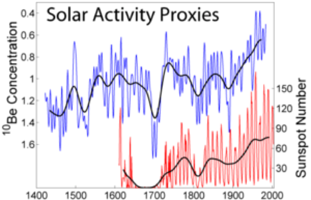
Because beryllium tends to exist in solutions below about pH 5.5 and rainwater above many industrialized areas can have a pH less than 5, it will dissolve and be transported to the Earth’s surface via rainwater. As the precipitation quickly becomes more alkaline, beryllium drops out of solution. Cosmogenic 10Be thereby accumulates at the soil surface, where its relatively long half-life permits a long residence time before decaying to 10B.

14C and 10Be are both produced by nuclear reactions of cosmic ray particles with the atmospheric gases. After production, their fate is very different (system effects). 10Be attaches to aerosols and is transported within a few years to the ground. 14C oxidizes to CO2 and enters the global carbon cycle, exchanging between atmosphere, biosphere, and the oceans.” width=”735″ height=”1024″> 14C and 10Be are both produced by nuclear reactions of cosmic ray particles with the atmospheric gases. After production, their fate is very different (system effects). 10Be attaches to aerosols and is transported within a few years to the ground. 14C oxidizes to CO2 and enters the global carbon cycle, exchanging between atmosphere, biosphere, and the oceans.
These variations have been successfully reproduced using models that employ magnetic flux continuity equations and observed sunspot numbers to quantify the emergence of magnetic flux from the top of the solar atmosphere and into the Heliosphere, showing that sunspot observations, geomagnetic activity and cosmogenic isotopes offer a convergent understanding of solar activity variations.
Dendroclimatology
Sunspot numbers over the past 11,400 years have been reconstructed using Carbon-14-based dendroclimatology.
Dendroclimatology is the science of determining past climates from trees. Tree rings are wider when conditions favor growth, narrower when times are difficult. Other properties of the annual rings, such as maximum latewood density (MXD) have been shown to be better proxies than simple ring width. By combining multiple tree-ring studies, sometimes with other climate proxy records, scientists have estimated many local climates for hundreds to thousands of years previous.
Tree rings are especially useful as climate proxies in that they are clearly demarked in annual increments and respond to multiple climatic effects such as temperature, precipitation, sunlight, and wind.
Non-climate factors include soil, tree age, fire, tree-to-tree competition, genetic differences, logging or other human disturbance, herbivore impact, pest outbreaks, disease, and carbon dioxide concentration.
The Milankovitch Cycles and Glaciation
During the last 650,000 years there have been seven cycles of glacial advance and retreat, with the abrupt end of the last ice age about 11,700 years ago marking the beginning of the modern climate era — and of human civilization. Most of these climate changes are attributed to very small variations in Earth’s orbit that change the amount of solar energy our planet receives.
The episodic nature of the Earth’s glacial and interglacial periods within the last couple of million years have been caused primarily by cyclical changes among variations in the Earth’s eccentricity, axial tilt, and precession, collectively known as the Milankovitch Cycles. They were named for Milutin Milankovitch, the Serbian astronomer who is generally credited with calculating their magnitude.
Variations in these three cycles create alterations in the seasonality of solar radiation reaching the Earth’s surface. These times of increased or decreased solar radiation directly influence the Earth’s climate system, particularly the advance and retreat of Earth’s glaciers. The three Milankovitch Cycles impact the seasonality and location of solar energy around the Earth, thus impacting contrasts between the seasons.
The 100,000 year Milankovitch cycle; eccentricity
Variations in the shape of Earth’s elliptical orbit.
The first of the three Milankovitch Cycles is eccentricity, the shape of the Earth’s orbit around the Sun. This constantly fluctuating orbital shape ranges between more and less elliptical (0 to 5% ellipticity) on a cycle of approximately 100,000 years. These oscillations, from more elliptic to less elliptic, are of prime importance to glaciation in that it alters the distance from the Earth to the Sun, thus changing the distance the Sun’s short wave radiation must travel to reach Earth, subsequently reducing or increasing the amount of radiation received at the Earth’s surface in different seasons.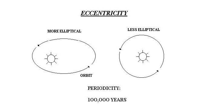
Today a difference of only about 3% occurs between aphelion (farthest point) and perihelion (closest point). This 3% difference in distance means that Earth experiences a 6% increase in received solar energy in January than in July. This 6% range of variability is not always the case, however. When the Earth’s orbit is most elliptical the amount of solar energy received at the perihelion would be in the range of 20% to 30% more than at aphelion. These continually changing amounts of received solar energy around the globe result in significant changes in the climate and glacial regimes of planet Earth. At present the orbital eccentricity is nearly at the minimum of its cycle.
The 41,000 year Milankovitch cycle: axial tilt
The precession of the equinoxes. Earth’s combined tilt and elliptical orbit around the Sun.
Axial tilt, the second of the three Milankovitch Cycles, is the inclination of the Earth’s axis of rotation in relation to the plane of its orbit around the Sun. Oscillations in the degree of the Earth’s axial tilt occur on a periodicity of 41,000 years from 21.5° to 24.5°.
Today the Earth’s axial tilt is about 23.5°, which largely accounts for our seasons. Because of the periodic variations of this angle the differences among the seasons on the Earth changes. With less axial tilt the Sun’s solar radiation is more evenly distributed between winter and summer. However, less tilt also increases the difference in radiation at the surface of the Earth between the equatorial and polar regions.
One hypothesis for Earth’s reaction to a smaller degree of axial tilt is that it would promote the growth of ice sheets. This response would be due to a warmer winter, in which warmer air would be able to hold more moisture, and subsequently produce a greater amount of snowfall. In addition, summer temperatures would be cooler, resulting in less melting of the winter’s accumulation. At present, axial tilt is in the middle of its range.
The 23,000 year Milankovitch cycle: precession
Cycle of the +/- 1.5° wobble in Earth’s orbit (tilt)
The third and final of the Milankovitch Cycles is precession, a slow wobble as the Earth turns on its axis. A consequence of the precession is a changing pole star.
The precession of Earth changes the orietation of the Earth and moves the “north” star over time to a different constellation in the night sky. The current pole star is Polaris located about one degree from the pole. The brilliant Vega in the constellation Lyra was the pole star around 12,000 BC and will be the pole star again around the year 14,000, however, it never comes closer than 5° to the true pole.
This top-like wobble, or precession, has a periodicity of 23,000 years.
When the axis of the Earth is tilted towards Vega the positions of the Northern Hemisphere winter and summer solstices will coincide with the aphelion and perihelion, respectively of the elliptical orbit. This means that the Northern Hemisphere will experience winter when the Earth is furthest from the Sun and summer when the Earth is closest to the Sun. This coincidence will result in greater seasonal contrasts. At present, the Earth is at perihelion very close to the winter solstice.
These variables are important because the Earth has an asymmetric distribution of landmasses, with virtually all, except Antarctica, located in the Northern Hemisphere.
At times when Northern Hemisphere summers are coolest—farthest from the Sun due to precession and greatest orbital eccentricity—and winters are warmest due to minimum tilt of the axis, snow can accumulate and cover broad areas of northern America and Europe. At present, only precession is in the glacial mode, with tilt and eccentricity not favorable to glaciation
Even when all of the orbital parameters favor glaciation, the increase in winter snowfall and decrease in summer melt would be barely enough to trigger glaciation, not to grow large ice sheets. Ice sheet growth requires the support of positive feedback loops, the most obvious of which is that large masses of ice and snow tend to reflect more radiation back into space thus cooling the climate and allowing glaciers to expand.
The Energy Budget of the Earth

The oceans of the Earth are vast, and owing to the specific heat of water, they contain vast amounts of thermal energy. Much of that energy is transferred around the earth through ocean currents. Some is transmitted to and from the atmosphere and controls local weather.
Ocean currents are driven by wind, the Coriolis effect, and thermohaline circulation which depends on density differences of waters entering the ocean.
The Winds
Wind is the primary force driving surface currents in the ocean. The sun heats the surface of the earth unevenly because of the shape and tilt of the earth. Warm air masses form where the sun’s radiation is most intense, at the equator. Cold air masses form at the poles, where the sun’s radiation is less intense. Warmer air masses rise into the atmosphere, creating areas of low pressure. As air masses cool high in the atmosphere, then sink and create areas of high pressure. The rising and sinking of air masses in the earth’s atmosphere create winds.
Rising warm, moist air at the equator travels northward and southward, cooling as it moves towards the poles. When this air reaches a certain cold temperature and density (at about 30 degrees N and S latitude), it sinks and creates an area of high pressure.
Where the air sinks, some travels towards the pole and some travels towards the equator. This air motion creates strong winds flowing from the west (“westerlies” and the northeast (trade winds) in the Northern Hemisphere. These dominant wind patterns drive oceanic currents.

Global winds
The Coriolis force and effect
Because the the earth rotates, rising air at the equator and sinking air at higher latitudes along a curved path relative to the surface of the earth as it flows creating winds in westerly and northeasterly directions because the earth is rotating beneath the air. This is known as the Coriolis effect.
Because of the direction of earth’s rotation, the Coriolis effect deflects air to the east as it flows towards the poles and towards the west as it flows towards the equator in the northern hemisphere. These deflected winds are known as “westerlies” and “northeasterly trade winds.”

coriolis effect on winds in Northern and Southern hemispheres
The Coriolis effect and ocean currents
Water set in motion by the wind is also deflected to the right in the Northern hemisphere and the left in the Southern hemisphere. At the surface in the Northern Hemisphere, water is transported at a net angle of 90 degrees to the right of the prevailing wind direction. This phenomenon is known as Ekman Transport, and is an important concept for understanding coastal upwelling and downwelling.
The motion of the winds and deflection of water towards the right (northern hemisphere) and left (southern hemisphere) of the prevailing wind directions generates large circular current systems in the world’s oceans known as gyres.
Deflection of water towards the center of the gyre due to the Coriolis effect causes water to “pile up” in the center of the gyre, creating an area of slightly higher elevation on the surface of the ocean. Gravity then pulls the water back down the slope to an area of lower elevation, fueling further rotation of the gyre.
Currents along the western side of gyres are called western boundary currents, while currents along the eastern side of gyres are called eastern boundary currents. The westerly flowing currents that are created where the North Pacific and South Pacific gyres meet are known as the equatorial currents
Western boundary currents flow deeper and stronger than eastern boundary currents. This means that cool, nutrient-rich water is closer to the surface in eastern boundary currents than western boundary currents. This results in the creation of rich upwelling zones in areas with eastern boundary currents, such as the California Current.

The major ocean gyres
Another consequence of the Earth’s eastward rotation and the resulting Coriolis effect is that the center of each of those gyres is offset toward the western edge of the ocean basin that confines it. Because the volume of water flowing toward the poles along the narrower western sides of the gyres is the same as that circulating back toward the Equator down the much broader eastern expanses, the constricted western currents are forced to flow much faster than their eastern counterparts. This results in such powerful currents as the Gulf Stream in the western North Atlantic, and the Kuroshio in the North Pacific.
The Gulf Stream starts roughly where the Gulf of Mexico narrows to form a channel between Cuba and the Florida Keys. From there the current flows northeast through the Straits of Florida between the mainland and the Bahamas, flowing at a substantial speed for some 400 miles.
The satellite photo shows the Gulf Stream, with the red being the warmest water and blue being the coolest.
While wind can play a role in shaping surface ocean currents, it is not the main or only factor. Wind plays virtually no role at all when it comes to deep ocean currents. The main drivers of ocean currents are the Coriolis force, density differences, tides and shoreline obstruction.
The Coriolis force is very weak, but when a lot of water is involved, such as in the ocean, the Coriolis force plays a large role. Because of the Coriolis force, the major ocean currents in the northern hemisphere tend to spiral clockwise and they tend to spiral counter-clockwise in the southern hemisphere.

Ocean current patterns. NOAA.
The Coriolis force is an inertial force that arises from the earth being in a rotating reference frame. It is very real in the rotating reference frame, but is not fundamental as it arises from the motion of the frame itself.
The Sargasso Sea

The Sargasso Sea is a region of the North Atlantic Ocean bounded by four currents forming an ocean gyre. Unlike all other regions called seas, it has no land boundaries. The Sargasso Sea is bounded on the west by the Gulf Stream, on the north by the North Atlantic Current, on the east by the Canary Current, and on the south by the North Atlantic Equatorial Current, all of which establish a clockwise-circulating system of ocean currents termed the North Atlantic Gyre. It lies between 70°and 40° W, and 20°to 35° N, and is approximately 1,100 km wide by 3,200 km long. Bermuda is near the western fringes of the Sargasso Sea.
It is distinguished from other parts of the Atlantic Ocean by its characteristic brown Sargassum seaweed and often calm blue water.
Geostrophic balance
Atmospheric winds and oceanic currents are driven by pressure gradients, from high towards low pressure. If the flow is maintained for a significant fraction of a day (i.e. several hours), then the Coriolis force, which acts on the moving fluids, air and water, will cause it to veer to the right of the pressure gradient in the northern hemisphere and to the left of the pressure gradient in the southern hemisphere. Given sufficient time, the flow will end up travelling at near right-angles to the pressure gradient, at which point, the Coriolis and the pressure gradient forces may be equal and opposite and the flow is said to be in “geostrophic balance”, and will persist in a rotational (cyclonic) pattern, counter-clockwise around a low pressure region in the northern hemisphere and clockwise in the southern. Around a high pressure zone the circulation is anti-cyclonic; clockwise in the northern hemisphere and counter-clockwise in the southern. It is geostrophic flows which cause storms and hurricanes to spin, and is the dynamics behind the “red spot” storm on the planet Jupiter.

The Coriolis Effect on storm cloud patterns. NASA.

Thermohaline circulation (THC
(THC) is a part of the large-scale ocean circulation that is driven by global density gradients created by surface heat and freshwater fluxes.The word thermohaline derives from thermo, referring to temperature, and haline, referring to salt content, factors which together determine the density of sea water.
Wind-driven surface currents such as the Gulf Stream travel polewards from the equatorial Atlantic Ocean, cooling en route and eventually sinking at high latitudes forming North Atlantic Deep Water. This colder denser water sinks and flows into the ocean basins. While the bulk of it upwells in the Southern Ocean, the oldest waters with a transit time of around 1000 years eventually upwell in the North Pacific establishing that the oceans of the Earth are a global system. On their journey, the water masses of the THC transport both energy in the form of heat and matter as solids, dissolved substances, and gases around the globe.

Thermohaline Circulation “Conveyor Belt” South polar view
The thermohaline circulation is sometimes called the ocean conveyor belt, the great ocean conveyor, or the global conveyor belt.

MAOC_2021_Nature
The Atlantic Meridional Overturning Circulation (AMOC) is is
a sensitive nonlinear system dependent on subtle thermohaline
density differences in the ocean. There is evidence that the AMOC is slowing
down and that the AMOC is presently in its weakest state in over 1,000 years. The AMOC is a a major mechanism for heat redistribution on Earth and an important factor in climate variability and change.
As continuous direct measurements of the AMOC started only in 20044 longer-term reconstruction must be based on proxy data: (1) reconstructions of surface or subsurface temperature patterns in the Atlantic Ocean that reflect the changes in ocean heat transport associated with the AMOC; (2) reconstructions of subsurface water mass properties, for example, the advance of the subpolar versus subtropical slope water, that reflect AMOC changes; and (3) evidence for physical changes in
deep-sea currents, such as those reflected by changes in sediment grain size. All three proxies can be influenced to some degree by factors
in addition to changes in the AMOC.
Despite the different locations, timescales and processes represented
by these proxies, they provide a consistent picture of the AMOC evolution since about AD 400. Before the nineteenth century, the AMOC was relatively stable. A decline in the AMOC, beginning during the nineteenth century occurred during the Little Ice Age of the 1790s. Around 1960 there began a phase of particularly rapid decline that is found in several, largely independent proxies followed by a short-lived recovery in the 1990s before a return to decline from the middle of the first decade of the 2000s.
All indices additionally show multi-decadal variability consistent with the evidence that climate changes continuously and always had with only relatively limited periuods of stability.
Temperature-density effects
Fresh waters are lighter than saline waters and warm waters are lighter than cold waters. The density of a water mass will determine whether it rises or sinks in the water column. Density differences create currents in the oceans.
Fluctuations in both temperature and salinity lead different regions of ocean water to have different densities. Higher temperatures, such as near the equator, cause a mass of water to expand and therefore drop in density. Also, lower salt content causes a mass of water to be lower in density. Gravity causes the more dense water to fall, pushing away the less dense water, which moves laterally and rises. Giant convection loops of ocean currents form as the lighter, warmer, and less salty regions of the oceans rise and flow to replace the heavier, cooler, and more salty regions of the oceans. The effect of density-driven currents is fundamentally a result of the interplay among solar heating, gravity, and salinity differences.
One possible effect of such changes in density is that warm events after glacial events deliver low-salinity, thus low-density, meltwaters into the ocean which tend to float rather than sink in areas where sinking (downwelling) normally takes place. This action interferes with total normal oceanic circulation; e.g. the Gulf Stream may be diverted eastward by meltwaters from the North American arctic, depriving England and northern Europe of the heat now moderating their climate.
If massive events such as floods of fresh water backed up in proglacial lakes were to spill into the ocean, then very rapid climate changes could take place by changing the ocean circulation patterns. At least two such events took place near the beginning of the present interglacial stage, with up to 4°–5° C rapid temperature swings in the Sargasso Sea.
The Carbon Cycle
 The carbon cycle is one of the biogeochemical cycles of the Earth that is most critical to the existence of life on the planet.
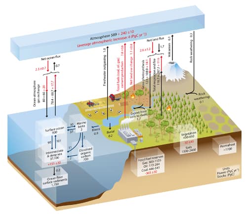
Fossil-fuel emissions, agricultural fertilization of croplands, and organic sewage discharges to aquatic systems have become part of and disturbed the carbon cycle. Land-use changes affect the uptake or release of carbon. Deforestation may result in weakening of the terrestrial carbon sink in the future. A change in the intensity of the thermohaline circulation could increase the ability of coastal marine waters to store atmospheric CO2.
Methods of estimating ancient temperatures
The geologic record contains many clues about former climates on Earth. Most of the proxies used to interpret past temperatures agree well enough to build a consensus about the more recent geologic past, and general acceptance of large-scale changes in the more distant past.
The geologic record of temperature variations/anomalies over the last two thousand years is rather well detailed.

There is still considerable detail back to the end of the last “Ice Age,” approximately 10,000 years ago.

Ice-core materials from mid- to low-latitude glaciers represent a time span of approximately 25,000 years and provide valuable insight into regional variation in climate patterns. Oxygen isotopes are used as a proxy for actual temperature.

The Greenland and Antrctic ice sheets today

Antarctic ice core stations

Climates throughout the Pleistocene geological epoch, often referred to colloquially as the Ice Age, which lasted from about 2,588,000 to 11,700 years ago are well documented; but the geologic records become progressively destroyed by erosion and tectonic cycling as time passes.
The accuracy of interpretations of past climates declines as we go farther back into the past.
Climates of 600 million years ago are less well documented, and those of billions of years ago are poorly documented.
Reconstructing paleoclimate
Reconstruction of paleoclimatic conditions based on the study of stable isotopes in ice core materials is one such proxy which is robust and not subject to uncertainties related to erosion, tectonism, or sedimentation processes. It has evolved into a well-recognized and powerful methodology.


O2 isotopes as paleoclimate proxies
Oxygen has three naturally occurring isotopes: 16O, 17O, and 18O, where the superscripts 16, 17 and 18 refer to the atomic mass. The most abundant oxygen isotope on Earth is 16O, with a small percentage of 18O and an even smaller percentage of 17O.
Oxygen isotope analysis determines the ratio of 18O to 16O present in a sample; then compares the calculated ratio of those masses to a standard to obtain information about the temperature at which the sample ice was formed.

Oxygen isotope ratio analysis
Oxygen isotopes, temperature, and weather
Because 18O is two neutrons “heavier” (more massive) than 16O and causes the water molecule in which it occurs to be heavier by that amount, it requires more energy to vaporize H18OH than H16OH (the water molecule is often written by organic chemists as HOH rather than H2O), and H18OH liberates more energy when it condenses. In addition, H16OH tends to diffuse more rapidly.
Because H16OH requires less energy to vaporize, and is more likely to diffuse to the liquid surface, the first water vapor formed during evaporation of liquid water is enriched in H16OH, and the residual liquid becomes enriched in H18OH.
When water vapor condenses into liquid, the “heavier” H18OH preferentially enters the liquid, while H16OH is concentrated in the remaining vapor.
As an air mass moves from a warm region to a cold region, water vapor condenses and is removed as precipitation. The precipitation removes H18OH, leaving progressively more H16OH-rich water vapor. This distillation process causes precipitation to have a lower ratio of 18O/16O as the temperature decreases. Additional factors can affect the efficiency of the distillation, such as the direct precipitation of ice crystals, rather than liquid water, at low temperatures.
Temperature and isotope ratios
Due to the intense precipitation that occurs in hurricanes, the H18OH is exhausted relative to the H16OH resulting in relatively low 18O/16O ratios. The subsequent uptake of hurricane rainfall in trees creates a record of the passing of hurricanes that can be used to create a historical record in the absence of human records.
When water evaporates in a time of cold temperatures relatively few atoms of the heavier 18O are picked up as compared to 16O, whereas in warm temperatures with more energy, more 18O is picked up. When that water is dropped on glaciers and preserved as ice, that ratio of isotopes is preserved. That permits the calculation of temperature from measuring the relative abundance of each isotope in ice core samples.
In geochemistry, paleoclimatology and paleoceanography δ18O is a measure of the ratio of stable isotopes oxygen-18 (18O) and oxygen-16 (16O). It is commonly used as a measure of the temperature of precipitation, as a measure of groundwater/mineral interactions, and as an indicator of processes that show isotopic fractionation, like methanogenesis. In paleosciences, 18O:16O data from corals, foraminifera and ice cores are used as a proxy for temperature.
Paleoclimate from benthic organisms
Using measurements of δ18O in benthic foraminifera from 57 globally distributed deep sea sediment cores taken as a proxy for the total global mass of glacial ice sheets, Lorraine Lisiecki was able to reconstruct the climate for the past five million years.
, A Pliocene-Pleistocene stack of 57 globally distributed benthic d18O records, Paleoceanography, 20, PA1003, doi:10.1029/2004PA001071) - Victor John Yannacone, jr")
Lisiecki, L. E., and M. E. Raymo (2005), A Pliocene-Pleistocene stack of 57 globally distributed benthic δ18O records, Paleoceanography, 20, PA1003, doi:10.1029/2004PA001071.
The stacked record of the 57 cores was orbitally tuned to an orbitally driven ice model, the Milankovitch cycles of 41 ky (obliquity), 26 ky (precession) and 100 ky (eccentricity), which are all assumed to cause orbital forcing of global ice volume. Over the past million years, there have been a number of very strong glacial maxima and minima, spaced by roughly 100 ky.

Glacial Cycles and benthic foraminifera
Paleoclimate from insects
In addition to techniques that may reveal paleoclimate information from marine settings, some lines of evidence are based exclusively on terrestrial organisms. Insects, specifically fossil beetles, provide such evidence.
A fossil beetle assemblage collected from northern Greenland demonstrates an unusual level of stasis through approximately 2 million years, even though the climate at that time was significantly warmer than that of today. The number of species remained relatively constant through several episodes of glaciation.
Beetles are highly mobile insects, and their most apparent response to variation in climate is migration from one location to another. This is well illustrated by the replacement (21,500 b.p.) of a forest fauna along the North American Laurentide ice sheet by a glacial fauna when temperatures were approximately 10°–12° C below current ones. When the ice sheet receded (approximately 12,500 b.p.), a forest fauna returned. Overall, beetles have survived global climatic changes due to their mobility.
Paleoclimate from stomatal index records
SI (Stomatal Index) values for birch trees dated (by radiocarbon) at 10,070 years correspond to CO2 levels of approximately 240 to 280 parts per million, volume (ppmv). Birch trees that are 9370 years old have SI values indicateing CO2 concentrations of 330–360 ppmv. Thus, these findings indicate an 80–90 ppmv variation in naturally occurring CO2 levels over a 700-year period. Additionally, SI data suggest a dramatic change of 65 ppmv CO2 levels in less than a century.
Several lines of evidence indicate that early to middle Miocene time, 23.03 to 5.333 million years ago, was one of the warmest periods of the entire Cenozoic, 66 to 0 million years ago. Fossil angiosperm materials of middle Eocene age showed elevated SI values indicating 450–500 ppmv for the CO2 level of the middle Eocene atmosphere.
Sea level changes
Sea surface level changes are measured today by specially purposed satellites.

The sea-level record approximates the “sawtooth” effect seen in the temperature records, that is, sharp warming episodes that gradually cool. The causes of this sawtooth effect are still being debated, but for glacial and interglacial episodes it may be the result of polar ocean freezing and cutting off moisture to feed continental glaciers, with rapid warming and sea-level rise as a consequence, or thermohaline circulation changes.
Over most of geologic history, long-term average sea level has been significantly higher than today. In the first graphic time moves from the Cambrian ~542 Ma ago on the left to the relatively recent Neogene ending ~2.58 Ma ago. Ma means “million years according to ISO rules.

Sea Level change through time
In this second graph covering the same period, the Cambrian is on the right and the Neogene is on the left. Otherwise the figures are equivalent.

Comparison of two sea level reconstructions during the last 500 Ma. The scale of change during the last glacial/interglacial transition is indicated with a black bar.
Various factors affect the volume or mass of the ocean and lead to long-term changes in eustatic sea level, the worldwide change of sea level elevation with time. The two primary influences are temperature because the density of water depends on its temperature, and the mass of water locked up on land and sea as fresh water in rivers, lakes, glaciers and polar ice caps.
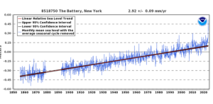
Modern era sea level changes
Data published by NOAA (National Oceanic & Atmospheric Administration) from the Battery at the tip of Manhattan Island. since the Civil War era. It is one of the longest continuous records we have of sea level rise. The rate of increase is about 10 inches per hundred years and shows no acceleration whatsoever despite substantial increases in CO2 during that time.
Ocean basin changes
Over long geological timescales, changes in the shape of oceanic basins and in land–sea distribution affect sea level. The shape of the ocean basins can change due to tectonic movement. If an ocean basin becomes larger, overall sea level will fall because there is no increase in the voume of ocean water. If the ocean basins become smaller, sea level rises accordingly. Orogeny (mountain building) and isostatic uplift are tectonic processes that change the sea level of an affected ocean basin

Orogeny affects the volume of ocean basins

Isostatic uplift affects the volume of ocean basins
Eustatic sea level changes
Eustatic change occurs when the sea level changes due to an alteration in the volume of water in the oceans or, alternatively, a change in the shape of an ocean basin and hence a change in the amount of water the sea can hold. Eustatic change is always a global effect.
During and after an ice age, eustatic change takes place. At the beginning of an ice age, the temperature falls and water is frozen and stored in glaciers inland, suspending the hydrological cycle. Water is taken out of the sea but not being replaced leading to an overall fall in sea level.
As an ice age ends, the temperature begins to rise and so the water stored in the glaciers reenters the hydrological cycle, the sea is replenished, and sea levels rise.
Evidence demonstrates that the last interglacial between approximately 135,000 and 115,000 years ago, maximum sea-level rise was about 6 meters (m) above the present sea level.
Since the Last Glacial Maximum about 20,000 years ago, sea level has risen by more than 125 m, with rates varying from tenths of a mm/yr to 10+mm/year.

During deglaciation between about 19,000 and 8,000 calendar years ago, sea level rose at extremely high rates as the result of the rapid melting of the British-Irish Sea, Fennoscandian, Laurentide, Barents-Kara, Patagonian, Innuitian ice sheets and parts of the Antarctic ice sheet. At the onset of deglaciation about 19,000 calendar years ago, a brief, at most 500-year long, glacio-eustatic event may have contributed as much as 10 m to sea level with an average rate of about 20 mm/yr. During the rest of the early Holocene, the rate of sea level rise varied from a low of about 6.0–9.9 mm/yr to as high as 30–60 mm/yr during brief periods of accelerated sea level rise.
Solid geological evidence, based largely upon analysis of deep cores of coral reefs, exists only for 3 major periods of accelerated sea level rise, called meltwater pulses, during the last deglaciation. They are Meltwater pulse 1A between circa 14,600 and 14,300 calendar years ago; Meltwater pulse 1B between circa 11,400 and 11,100 calendar years ago; and Meltwater pulse 1C between 8,200 and 7,600 calendar years ago. Meltwater pulse 1A was a 13.5 m rise over about 290 years centered at 14,200 calendar years ago and Meltwater pulse 1B was a 7.5 m rise over about 160 years centered at 11,000 years calendar years ago.
In sharp contrast, the period between 14,300 and 11,100 calendar years ago, which includes the Younger Dryas interval, was an interval of reduced sea level rise at about 6.0–9.9 mm/yr. Meltwater pulse 1C was centered at 8,000 calendar years and produced a rise of 6.5 m in less than 140 years. Such rapid rates of sea level rising during meltwater events clearly implicate major ice-loss events related to ice sheet collapse. The primary source may have been meltwater from the Antarctic ice sheet.

Other studies suggest a Northern Hemisphere source for the meltwater in the Laurentide ice sheet.

The Laurentide Ice Sheet was a massive sheet of ice that covered millions of square kilometers, including most of Canada and a large portion of the northern United States, multiple times during the Quaternary glacial epochs— from 2.588 ± 0.005 million years ago to the present.
The last advance covered most of northern North America between c. 95,000 and c. 20,000 years before the present day, and among other geomorphological effects, gouged out the five Great Lakes and the hosts of smaller lakes of the Canadian shield. These lakes extend from the eastern Northwest Territories, through most of northern Canada, and the upper Midwestern United States (Minnesota, Wisconsin, and Michigan) to the Finger Lakes, through Lake Champlain and Lake George areas of New York, across the northern Appalachians into and through all of New England and Nova Scotia.
At times, the ice sheet’s southern margin included the present-day sites of northeastern coastal towns and cities such as Portsmouth, New Hampshire, Boston, and New York City, and Great Lakes coastal cities and towns as far south as Chicago and St. Louis, Missouri, and then followed quite precisely the present course of the Missouri River up to the northern slopes of the Cypress Hills, beyond which it merged with the Cordilleran Ice Sheet. The ice coverage extended approximately as far south as 38 degrees latitude in the mid-continent.

Recently, it has become widely accepted that late Holocene, 3,000 calendar years ago to present, sea level was nearly stable prior to an acceleration in the rate of rise that is variously dated between 1850 and 1900 AD. Late Holocene rates of sea level rise have been estimated using evidence from archaeological sites and late Holocene tidal marsh sediments, combined with tide gauge and satellite records and geophysical modeling. This research included studies of Roman wells in Caesarea and of Roman piscinae (fish ponds) in Italy. These methods in combination suggest a mean eustatic component of 0.07 mm/yr for the last 2000 years.
Since 1880, however, the ocean has begun to rise briskly: a total of 210 mm (8.3 in) through 2009 causing extensive erosion worldwide.
The origins of the CO2 Controversy
In 1896, Svante Arrhenius, started the debate on the effect of atmospheric carbon dioxide concentration on global temperature with his original work on atmospheric gases, On the Influence of Carbonic Acid upon the Temperature of the Ground in which he stated that “if the quantity of carbonic acid [carbon dioxide] increases in geometric progression, the augmentation of the temperature will increase nearly in arithmetic progression.”
Arrhenius, who first identified carbon dioxide as a “greenhouse gas” in 1896, in the same paper also showed that carbon dioxide loses effectiveness logarithmically with increasing concentration so that the greenhouse effect attributable to the rise from 100 to 200 parts per million (ppm) is much greater than during the rise from 300 to 400 ppm. A part per million has been likened to a jigger of vermouth in a railroad car full of gin—the recipe for a very very dry martini.
An uncontrolled experiment on Western Civilization
The position of the United Nations IPCC (Intergovernmental Panel on Climate Change) claims that carbon dioxide from human activities, particularly industrial activity and transportation is responsible for global “warming” and relies for that opinion on numeric computer models.
The ever-increasing concentration of carbon dioxide in the atmosphere which is assumed to be the result of human activity is presumed to drive global temperature upwards and make global climate warmer. The remedy for this “dangerous crisis” is to eliminate the use of fossil fuels because their combustion releases carbon dioxide into the atmosphere yet there is no substantial credible evidence that the tiny contribution of human activity to the level of caron dioxide in the atmosphere is a significant contributor to global climate change.